Julia is a high-level, dynamic programming language, designed to give users the speed of C/C++ while remaining as easy to use as Python. This means that developers can solve problems faster and more effectively.
Julia is great for computational complex problems. Many early adopters of Julia were concentrated in scientific domains like Chemistry, Biology, and Machine Learning.
This said, Julia is general-purpose language and can be used for tasks like Web Development, Game Development, and more. Many view Julia as the next-generation language for Machine Learning and Data Science, including the CEO of Shopify (among many others):
How to Download the Julia Programming Language ⤵️
There are two main ways to run Julia: via a .jl file in an IDE like VS Code or command by command in the Julia REPL (Read Evaluate Print Loop). In this guide, we will mainly use the Julia REPL. Before you can use either, you will need to download Julia:
or just head to: https://julialang.org/downloads/
After you have Julia installed, you should be able to launch it and see:
Julia 1.7 REPL after install
Julia Programming Language Basics for Beginners
Before we can use Julia for all of the exciting things it was built for like Machine Learning or Data Science, we first need to get familiar with the basics of the language.
We will start by going over variables, types, and conditionals. Then, we will talk about loops, functions, and packages. Last, we’ll touch on more advanced concepts like structs and talk about additional learning resources.
This is going to be a whirlwind tour so strap in and get ready! It is also worth noting that this tutorial assumes you have some basic familiarity with programming. If you don't, check out this course on an Intro to Julia for Nervous Beginners.
An Introduction to Julia Variables and Types ⌨️
In Julia, variables are dynamically typed, meaning that you do not need to specify the variable's type when you create it.
julia> a = 10 # Create the variable "a" and assign it the number 10
10
julia> a + 10 # Do a basic math operation using "a"
20(Note that in code snippets, when you see julia> it means the code is being run in the REPL)
Just like we defined a variable above and assigned it an integer (whole number), we can also do something similar for strings and other variable types:
julia> my_string = "Hello freeCodeCamp" # Define a string variable
"Hello freeCodeCamp"
julia> balance = 238.19 # Define a float variable
238.19
When creating variables in Julia, the variable name will always go on the left-hand side, and the value will always go on the right-hand side after the equals sign. We can also create new variables based on the values of other variables:
julia> new_balance = balance + a
248.19
Here we can see that the new_balance is now the sum (total) of 238.19 and 10. Note further that the type of new_balance is a float (number with decimal place precision) because when we add a float and int together, we automatically get the type with higher precision, which in this case is a float. We can confirm this by doing:
julia> typeof(new_balance)
Float64
Due to the nature of dynamic typing, variables in Julia can also change type. This means that at one point, holder_balance could be a float, and then later on it could be a string:
julia> holder_balance = 100.34
100.34
julia> holder_balance = "The Type has changed"
"The Type has changed"
julia> typeof(holder_balance)
String
You may also be excited to know that variable names in Julia are very flexible, in fact, you can do something like:
julia> 😀 = 10
10
julia> 🥲 = -10
-10
julia> 😀 + 🥲
0
On top of emoji variable names, you can also use any other Unicode variable name which is very helpful when you are trying to represent mathematical ideas. You can access these Unicode variables by doing a \ and then typing the name, followed by pressing tab:
julia> \sigma # press tab and it will render the symbol
julia> σ = 10 # set sigma equal to 10
Overall, the variable system in Julia is flexible and provides a huge set of features that make writing Julia code easy while still being expressive. If you want to learn more about variables in Julia, check out the Julia documentation: https://docs.julialang.org/en/v1/manual/variables/
How to Write Conditional Statements in Julia 🔀
In programming, you often need to check certain conditions in order to make sure that specific lines of code run. For example, if you write a banking program, you might only want to let someone withdraw money if the amount they are trying to withdraw is less than the amount they have present in their account.
Let us look at a basic example of a conditional statement in Julia:
julia> bank_balance = 4583.11
4583.11
julia> withdraw_amount = 250
250
julia> if withdraw_amount <= bank_balance
bank_balance -= withdraw_amount
print("Withdrew ", withdraw_amount, " from your account")
end
Withdrew 250 from your account
Let us take a closer look here at some parts of the if statement that might differ from other code you have seen: First, we use no : to denote the end of the line and we also are not required to use () around the statement (though it is encouraged). Next, we don't use {} or the like to denote the end of the conditional, instead, we use the end keyword.
Just like we used the if statement, we can chain it with an else or an elseif:
julia> withdraw_amount = 4600
4600
julia> if withdraw_amount <= bank_balance
bank_balance -= withdraw_amount
print("Withdrew ", withdraw_amount, " from your account")
else
print("Insufficent balance")
end
Insufficent balance
You can read more about control flow and conditional expressions in the Julia documentation: https://docs.julialang.org/en/v1/manual/control-flow/#man-conditional-evaluation
How to use Loops in Julia 🔂
There are two main types of loops in Julia: a for loop and a while loop. As is the same with other languages, the biggest difference is that in a for loop, you are going through a pre-defined number of items whereas, in a while loop, you are iterating until some condition is changed.
Syntactically, the loops in Julia look very similar in structure to the if conditionals we just looked at:
julia> greeting = ["Hello", "world", "and", "welcome", "to", "freeCodeCamp"] # define greeting, an array of strings
6-element Vector{String}:
"Hello"
"world"
"and"
"welcome"
"to"
"freeCodeCamp"
julia> for word in greeting
print(word, " ")
end
Hello world and welcome to freeCodeCamp
In this example, we first defined a new type: a vector (also called an array). This array is holding a bunch of strings we defined. The behavior is very similar to that of arrays in other languages but it is worth noting that arrays are mutable (meaning you can change the number of items in the array after you create it).
Again, when we look at the structure of the for loop, you can see that we are iterating through the greeting variable. Each time through, we get a new word (in this case) from the array and assign it to a temporary variable word which we then print out. You will notice that the structure of this loop looks similar to the if statement and again uses the end keyword.
Now that we explored for loops, let us switch gears and take a look at a while loop in Julia:
julia> while user_input != "End"
print("Enter some input, or End to quit: ")
user_input = readline() # Prompt the user for input
end
Enter some input, or End to quit: hi
Enter some input, or End to quit: test
Enter some input, or End to quit: no
Enter some input, or End to quit: End
For this while loop, we set it up so that it will run indefinitely until the user typed the word "End". As you have now seen it a few times, the structure of the loop should start to look familiar.
If you want to see some more examples of loops in Julia, you can check out the Julia Documentation's section on loops: https://docs.julialang.org/en/v1/manual/control-flow/#man-loops
How to use Functions in Julia
Functions are used to create multiple lines of code, chained together, and accessible when you reference a function name. First, let us look at an example of a basic function:
julia> function greet()
print("Hello new Julia user!")
end
greet (generic function with 1 method)
julia> greet()
Hello new Julia user!
Functions can also take arguments, just like in other languages:
julia> function greetuser(user_name)
print("Hello ", user_name, ", welcome to the Julia Community")
end
greetuser (generic function with 1 method)
julia> greetuser("Logan")
Hello Logan, welcome to the Julia Community
In this example, we take in one argument, and then add its value to the print out. But what if we don't get a string?
julia> greetuser(true)
Hello true, welcome to the Julia Community
In this case, since we are just printing, the function continues to work despite not taking in a string anymore and instead of taking a boolean value (true or false). To prevent this from occurring, we can explicitly type the input arguments as follows:
julia> function greetuser(user_name::String)
print("Hello ", user_name, ", welcome to the Julia Community")
end
greetuser (generic function with 2 methods)
julia> greetuser("Logan")
Hello Logan, welcome to the Julia Community
So now the function is defined to take in only a string. Let us test this out to make sure we can only call the function with a string value:
julia> greetuser(true)
Hello true, welcome to the Julia Community
Wait a second, why is this happening? We re-defined the greetuser function, it should not take true anymore.
What we are experiencing here is one of the most powerful underlying features of Julia: Multiple Dispatch. Julia allows us to define functions with the same name and number of arguments but that accept different types. This means we can build either generic or type specific versions of functions which helps immensely with code readability since you don't need to handle every scenario in one function.
We should quickly confirm that we actually defined both functions:
julia> methods(greetuser)
# 2 methods for generic function "greetuser":
[1] greetuser(user_name::String) in Main at REPL[34]:1
[2] greetuser(user_name) in Main at REPL[30]:1
The built-in methods function is perfect for this and it tells us we have two functions defined, with the only difference being one takes in any type, and the other takes in just a string.
It is worth noting that since we defined a specialized version that accepts just a string, anytime we call the function with a string it will call the specialized version. The more generic function will not be called when a string is passed in.
Next, let us talk about returning values from a function. In Julia, you have two options, you can use the explicit return keyword, or you can opt to do it implicitly by having the last expression in the function serve as the return value like so:
julia> function sayhi()
"This is a test"
"hi"
end
sayhi (generic function with 1 method)
julia> sayhi()
"hi"
In the above example, the string value "hi" is returned from the function since it is the last expression and there is no explicit return statement. You could also define the function like:
julia> function sayhi()
"This is a test"
return "hi"
end
sayhi (generic function with 1 method)
julia> sayhi()
"hi"
In general, from a readability standpoint, it makes sense to use the explicit return statement in case someone reading your code does not know about the implicit return behavior in Julia functions.
Another useful functions feature is the ability to provide optional arguments:
julia> function sayhello(response="hello")
return response
end
sayhello (generic function with 2 methods)
julia> sayhello()
"hello"
julia> sayhello("hi")
"hi"
In this example, we define response as an optional argument so that we can either allow it to use the default behavior we defined or we can manually override it when necessary. These examples just scratch the surface on what is possible with functions in Julia. If you want to read more about all the cool things you can do, check out: https://docs.julialang.org/en/v1/manual/functions/
How to use Packages in Julia 📦
The Julia package manager and package ecosystem are some of the most important features of the language. I actually wrote an entire article on why it is one of the most underrate features of the language.
With that said, there are two ways to interact with packages in Julia: via the REPL or using the Pkg package. We will mostly focus on the REPL in this post since it is much easier to use in my experience.
After you have Julia installed, you can enter the package manager from the REPL by typing ].
Pkg mode in the Julia REPL
Now that we are in the package manager, there are a few things we commonly want to do:
Add a package
Remove a package
Check what is already installed
If you want to see all the possible commands in the REPL, simply enter Pkg mode by typing ] and then type ? followed by the enter / return key.
How to Add Julia Packages ➕
Let’s add our first package, Example.jl . To do so, we can run:
(@v1.7) pkg> add Example
which should provide output that looks something like:
(@v1.7) pkg> add Example
Updating registry at `~/.julia/registries/General`
Updating git-repo `https://github.com/JuliaRegistries/General.git`
Updating registry at `~/.julia/registries/JuliaPOMDP`
Updating git-repo `https://github.com/JuliaPOMDP/Registry`
Resolving package versions...
Installed Example ─ v0.5.3
Updating `~/.julia/environments/v1.7/Project.toml`
[7876af07] + Example v0.5.3
Updating `~/.julia/environments/v1.7/Manifest.toml`
[7876af07] + Example v0.5.3
Precompiling project...
1 dependency successfully precompiled in 1 seconds (69 already precompiled)
(@v1.7) pkg>
For space reasons, I will skip further outputs under the assumption that you are following along with me.
How to Check the Package Status in Julia 🔍
Now that we think we have a package installed, let’s doublecheck if it is really there by typing status (or st for shorthand) into the package manager:
(@v1.7) pkg> st
Status `~/.julia/environments/v1.7/Project.toml`
[7876af07] Example v0.5.3
[587475ba] Flux v0.12.8
Here we can see I have two packages installed, Flux and Example. It also gives me the path to the file which manages my current environment (in this case, global Julia v1.7) along with the package versions I have installed.
How to Remove a Julia package 📛
If I wanted to remove a package from my active environment, like Flux, I can simply type remove Flux (or rm as the shorthand):
(@v1.7) pkg> rm Flux
Updating `~/.julia/environments/v1.7/Project.toml`
[587475ba] - Flux v0.12.8
A quick status afterward shows this was successful:
(@v1.7) pkg> st
Status `~/.julia/environments/v1.7/Project.toml`
[7876af07] Example v0.5.3
We now know the very basics of working with packages. But we have committed a major programming crime, using our global package environment.
How to Use Julia Packages 📦
Now that we have gone over how to manage packages, let’s explore how to use them. Quite simply, you just need to type using packageName to use a specific package you want. One of my favorite new features in Julia 1.7 (highlighted in this blog post) is shown below:
If you recall, we removed the Flux package, and of course, I forgot this so I went to use it and load it in by typing using Flux. The REPL automatically prompts me to install it via a simple "y/n" prompt. This is a small feature but saves a tremendous amount of time and potential confusion.
It is worth noting that there are two ways to access a package's exported functions: via the using keyword and the import keyword. The big difference is that using automatically brings all of the functions into the current namespace (for which you can think about as a big list of functions which Julia knows the definitions) whereas import gives you access to all of the functions but you have to prefix the function with the package name like: Flux.gradient() where Flux is the name of the package and gradient() is the name of a function.
How to use Structs in Julia?
Julia does not have Object Orientated Programming (OOP) paradigms built into the language like classes. However, structs in Julia can be used similar to classes to create custom objects and types. Below, we will show a basic example:
julia> mutable struct dog
           breed::String
           paws::Int
           name::String
           weight::Float64
       end

julia> my_dog = dog("Australian Shepard", 4, "Indy", 34.0)
dog("Australian Shepard", 4, "Indy", 34.0)

julia> my_dog.name
"Indy"
In this example, we define a struct to represent a dog. In the struct, we define four attributes which make up the dog object. In the lines after that, we show the code to actually create a dog object and then access some of its attributes. Note that you need not specify the types of the attributes, you could leave it more open. For this example, we defined explicit types to highlight that feature.
You will notice that similar to classes in Python (and other languages), we did not define an explicit constructor to create the dog object. We can, however, define one if that would be useful to use:
julia> mutable struct dog
           breed::String
           paws::Int
           name::String
           weight::Float64

           function dog(breed, name, weight, paws=4)
               new(breed, paws, name, weight)
           end
       end

julia> new_dog = dog("German Shepard", "Champ", 46)
dog("German Shepard", 4, "Champ", 46.0)
Here we defined a constructor and used the special keyword new in order to create the object at the end of the function. You can also create getters and setters specifically for the dog object by doing the following:
julia> function get_name(dog_obj::dog)
           print("The dogs's name is: ", dog_obj.name)
       end
get_name (generic function with 1 method)

julia> get_name(new_dog)
The dogs's name is: Champ
In this example, the get_name function only takes an object of type dog. If you try to pass in something else, it will error out:
julia> get_name("test")
ERROR: MethodError: no method matching get_name(::String)
Closest candidates are:
  get_name(::dog) at REPL[61]:1
Stacktrace:
 [1] top-level scope
   @ REPL[63]:1
It is worth noting that we also defined the struct to be mutable initially so that we could change the field values after we created the object. You omit the keyword mutable if you want the objects initial state to persist.
Structs in Julia not only allow us to create object's, we also are defining a custom type in the process:
julia> typeof(new_dog)
dog
In general, structs are used heavily across the Julia ecosystem and you can learn more about them in the docs: https://docs.julialang.org/en/v1/base/base/#struct
Additional Julia Programming Learning Resources 📚
I hope that this tutorial helped get you up to speed on many of the core ideas of the Julia language. With that said, I know that there are still gaps as this is an extended but non-comprehensive guide. To learn more about Julia, you can check out the learning tab on the Julia website: https://julialang.org/learning/ which has guided courses, YouTube videos, and mentored practice problems.
https://juliabyexample.helpmanual.io/
Set of unofficial examples of Julia the high-level, high-performance dynamic programming language for technical computing.
Below are a series of examples of common operations in Julia. They assume you already have Julia installed and working
(the examples are currently tested with Julia v1.0.5).
Hello World
The simplest possible script.
println("hello world")
With Julia installed and added to your path
this script can be run by julia hello_world.jl, it can also be run from REPL by typing
include("hello_world.jl"), that will evaluate all valid expressions in that file and return the last output.
Simple Functions
The example below shows two simple functions, how to call them and print the results.
Further examples of number formatting are shown below.
# function to calculate the volume of a sphere
function sphere_vol(r) # julia allows Unicode names (in UTF-8 encoding) # so either "pi" or the symbol π can be used return 4/3*pi*r^3
end
# functions can also be defined more succinctly
quadratic(a, sqr_term, b) = (-b + sqr_term) / 2a
# calculates x for 0 = a*x^2+b*x+c, arguments types can be defined in function definitions
function quadratic2(a::Float64, b::Float64, c::Float64) # unlike other languages 2a is equivalent to 2*a # a^2 is used instead of a**2 or pow(a,2) sqr_term = sqrt(b^2-4a*c) r1 = quadratic(a, sqr_term, b) r2 = quadratic(a, -sqr_term, b) # multiple values can be returned from a function using tuples # if the return keyword is omitted, the last term is returned r1, r2
end
vol = sphere_vol(3)
# @printf allows number formatting but does not automatically append the \n to statements, see below
using Printf
@printf "volume = %0.3f\n" vol
#> volume = 113.097
quad1, quad2 = quadratic2(2.0, -2.0, -12.0)
println("result 1: ", quad1)
#> result 1: 3.0
println("result 2: ", quad2)
#> result 2: -2.0
Strings Basics
Collection of different string examples (string indexing is the same as array indexing: see below).
# strings are defined with double quotes
# like variables, strings can contain any unicode character
s1 = "The quick brown fox jumps over the lazy dog α,β,γ"
println(s1)
#> The quick brown fox jumps over the lazy dog α,β,γ
# println adds a new line to the end of output
# print can be used if you dont want that:
print("this")
#> this
print(" and")
#> and
print(" that.\n")
#> that.
# chars are defined with single quotes
c1 = 'a'
println(c1)
#> a
# the ascii value of a char can be found with Int():
println(c1, " ascii value = ", Int(c1))
#> a ascii value = 97
println("Int('α') == ", Int('α'))
#> Int('α') == 945
# so be aware that
println(Int('1') == 1)
#> false
# strings can be converted to upper case or lower case:
s1_caps = uppercase(s1)
s1_lower = lowercase(s1)
println(s1_caps, "\n", s1_lower)
#> THE QUICK BROWN FOX JUMPS OVER THE LAZY DOG Α,Β,Γ
#> the quick brown fox jumps over the lazy dog α,β,γ
# sub strings can be indexed like arrays:
# (show prints the raw value)
show(s1[11]); println()
#> 'b'
# or sub strings can be created:
show(s1[1:10]); println()
#> "The quick "
# end is used for the end of the array or string
show(s1[end-10:end]); println()
#> "dog α,β,γ"
# julia allows string Interpolation:
a = "welcome"
b = "julia"
println("$a to $b.")
#> welcome to julia.
# this can extend to evaluate statements:
println("1 + 2 = $(1 + 2)")
#> 1 + 2 = 3
# strings can also be concatenated using the * operator
# using * instead of + isn't intuitive when you start with Julia,
# however people think it makes more sense
s2 = "this" * " and" * " that"
println(s2)
#> this and that
# as well as the string function
s3 = string("this", " and", " that")
println(s3)
#> this and that
String: Converting and formatting
# strings can be converted using float and int:
e_str1 = "2.718"
e = parse(Float64, e_str1)
println(5e)
#> 13.59
num_15 = parse(Int, "15")
println(3num_15)
#> 45
# numbers can be converted to strings and formatted using printf
using Printf
@printf "e = %0.2f\n" e
#> e = 2.72
# or to create another string sprintf
e_str2 = @sprintf("%0.3f", e)
# to show that the 2 strings are the same
println("e_str1 == e_str2: $(e_str1 == e_str2)")
#> e_str1 == e_str2: true
# available number format characters are f, e, a, g, c, s, p, d:
# (pi is a predefined constant; however, since its type is
# "MathConst" it has to be converted to a float to be formatted)
@printf "fix trailing precision: %0.3f\n" float(pi)
#> fix trailing precision: 3.142
@printf "scientific form: %0.6e\n" 1000pi
#> scientific form: 3.141593e+03
@printf "float in hexadecimal format: %a\n" 0xff
#> float in hexadecimal format: 0xf.fp+4
@printf "fix trailing precision: %g\n" pi*1e8
#> fix trailing precision: 3.14159e+08
@printf "a character: %c\n" 'α'
#> a character: α
@printf "a string: %s\n" "look I'm a string!"
#> a string: look I'm a string!
@printf "right justify a string: %50s\n" "width 50, text right justified!"
#> right justify a string:width 50, text right justified!
@printf "a pointer: %p\n" 100000000
#> a pointer: 0x0000000005f5e100
@printf "print an integer: %d\n" 1e10
#> print an integer: 10000000000
String Manipulations
s1 = "The quick brown fox jumps over the lazy dog α,β,γ"
# search returns the first index of a char
i = findfirst(isequal('b'), s1)
println(i)
#> 11
# the second argument is equivalent to the second argument of split, see below
# or a range if called with another string
r = findfirst("brown", s1)
println(r)
#> 11:15
# string replace is done thus:
r = replace(s1, "brown" => "red")
show(r); println()
#> "The quick red fox jumps over the lazy dog α,β,γ"
# search and replace can also take a regular expressions by preceding the string with 'r'
r = findfirst(r"b[\w]*n", s1)
println(r)
#> 11:15
# again with a regular expression
r = replace(s1, r"b[\w]*n" => "red")
show(r); println()
#> "The quick red fox jumps over the lazy dog α,β,γ"
# there are also functions for regular expressions that return RegexMatch types
# match scans left to right for the first match (specified starting index optional)
r = match(r"b[\w]*n", s1)
println(r)
#> RegexMatch("brown")
# RegexMatch types have a property match that holds the matched string
show(r.match); println()
#> "brown"
# eachmatch returns an iterator over all the matches
r = eachmatch(r"[\w]{4,}", s1)
for i in r print("\"$(i.match)\" ") end
#> "quick" "brown" "jumps" "over" "lazy"
println()
r = collect(m.match for m = eachmatch(r"[\w]{4,}", s1))
println(r)
#> SubString{String}["quick", "brown", "jumps", "over", "lazy"]
# a string can be repeated using the repeat function,
# or more succinctly with the ^ syntax:
r = "hello "^3
show(r); println() #> "hello hello hello "
# the strip function works the same as python:
# e.g., with one argument it strips the outer whitespace
r = strip("hello ")
show(r); println() #> "hello"
# or with a second argument of an array of chars it strips any of them;
r = strip("hello ", ['h', ' '])
show(r); println() #> "ello"
# (note the array is of chars and not strings)
# similarly split works in basically the same way as python:
r = split("hello, there,bob", ',')
show(r); println() #> SubString{String}["hello", " there", "bob"]
r = split("hello, there,bob", ", ")
show(r); println() #> SubString{String}["hello", "there,bob"]
r = split("hello, there,bob", [',', ' '], limit=0, keepempty=false)
show(r); println() #> SubString{String}["hello", "there", "bob"]
# (the last two arguements are limit and include_empty, see docs)
# the opposite of split: join is simply
r = join(collect(1:10), ", ")
println(r) #> 1, 2, 3, 4, 5, 6, 7, 8, 9, 10
Arrays
function printsum(a) # summary generates a summary of an object println(summary(a), ": ", repr(a))
end
# arrays can be initialised directly:
a1 = [1,2,3]
printsum(a1)
#> 3-element Array{Int64,1}: [1, 2, 3]
# or initialised empty:
a2 = []
printsum(a2)
#> 0-element Array{Any,1}: Any[]
# since this array has no type, functions like push! (see below) don't work
# instead arrays can be initialised with a type:
a3 = Int64[]
printsum(a3)
#> 0-element Array{Int64,1}: Int64[]
# ranges are different from arrays:
a4 = 1:20
printsum(a4)
#> 20-element UnitRange{Int64}: 1:20
# however they can be used to create arrays thus:
a4 = collect(1:20)
printsum(a4)
#> 20-element Array{Int64,1}: [1, 2, 3, 4, 5, 6, 7, 8, 9, 10, 11, 12, 13, 14,
#> 15, 16, 17, 18, 19, 20]
# arrays can also be generated from comprehensions:
a5 = [2^i for i = 1:10]
printsum(a5)
#> 10-element Array{Int64,1}: [2, 4, 8, 16, 32, 64, 128, 256, 512, 1024]
# arrays can be any type, so arrays of arrays can be created:
a6 = (Array{Int64, 1})[]
printsum(a6)
#> 0-element Array{Array{Int64,1},1}: Array{Int64,1}[]
# (note this is a "jagged array" (i.e., an array of arrays), not a multidimensional array,
# these are not covered here)
# Julia provided a number of "Dequeue" functions, the most common
# for appending to the end of arrays is
# ! at the end of a function name indicates that the first argument is updated.
push!(a1, 4)
printsum(a1)
#> 4-element Array{Int64,1}: [1, 2, 3, 4]
# push!(a2, 1) would cause error:
push!(a3, 1)
printsum(a3) #> 1-element Array{Int64,1}: [1]
#> 1-element Array{Int64,1}: [1]
push!(a6, [1,2,3])
printsum(a6)
#> 1-element Array{Array{Int64,1},1}: Array{Int64,1}[[1, 2, 3]]
# using repeat() to create arrays
# you must use the keywords "inner" and "outer"
# all arguments must be arrays (not ranges)
a7 = repeat(a1,inner=[2],outer=[1])
printsum(a7)
#> 8-element Array{Int64,1}: [1, 1, 2, 2, 3, 3, 4, 4]
a8 = repeat(collect(4:-1:1),inner=[1],outer=[2])
printsum(a8)
#> 8-element Array{Int64,1}: [4, 3, 2, 1, 4, 3, 2, 1]
Error Handling
# try, catch can be used to deal with errors as with many other languages
try push!(a,1)
catch err showerror(stdout, err, backtrace());println()
end
#> UndefVarError: a not defined
#> Stacktrace:
#> [1] top-level scope at C:\JuliaByExample\src\error_handling.jl:5
#> [2] include at .\boot.jl:317 [inlined]
#> [3] include_relative(::Module, ::String) at .\loading.jl:1038
#> [4] include(::Module, ::String) at .\sysimg.jl:29
#> [5] exec_options(::Base.JLOptions) at .\client.jl:229
#> [6] _start() at .\client.jl:421
println("Continuing after error")
#> Continuing after error
Multidimensional Arrays
Julia has very good multidimensional array capabilities.
Check out the manual.
# repeat can be useful to expand a grid
# as in R's expand.grid() function:
m1 = hcat(repeat([1,2],inner=[1],outer=[3*2]),
repeat([1,2,3],inner=[2],outer=[2]),
repeat([1,2,3,4],inner=[3],outer=[1]))
printsum(m1)
#> 12×3 Array{Int64,2}: [1 1 1; 2 1 1; 1 2 1; 2 2 2; 1 3 2; 2 3 2; 1 1 3; 2 1 3;
#> 1 2 3; 2 2 4; 1 3 4; 2 3 4]
# for simple repetitions of arrays,
# use repeat
m2 = repeat(m1,1,2) # replicate a9 once into dim1 and twice into dim2
println("size: ", size(m2))
#> size: (12, 6)
m3 = repeat(m1,2,1) # replicate a9 twice into dim1 and once into dim2
println("size: ", size(m3))
#> size: (24, 3)
# Julia comprehensions are another way to easily create
# multidimensional arrays
m4 = [i+j+k for i=1:2, j=1:3, k=1:2] # creates a 2x3x2 array of Int64
m5 = ["Hi Im # $(i+2*(j-1 + 3*(k-1)))" for i=1:2, j=1:3, k=1:2]
# expressions are very flexible
# you can specify the type of the array by just
# placing it in front of the expression
import LegacyStrings
m5 = LegacyStrings.ASCIIString["Hi Im element # $(i+2*(j-1 + 3*(k-1)))" for i=1:2, j=1:3, k=1:2]
printsum(m5)
#> 2×3×2 Array{LegacyStrings.ASCIIString,3}: LegacyStrings.ASCIIString[
#> "Hi Im element # 1" "Hi Im element # 3" "Hi Im element # 5";
#> "Hi Im element # 2" "Hi Im element # 4" "Hi Im element # 6"]
#>
#> LegacyStrings.ASCIIString["Hi Im element # 7" "Hi Im element # 9"
#> "Hi Im element # 11"; "Hi Im element # 8" "Hi Im element # 10" "Hi Im element # 12"]
# Array reductions
# many functions in Julia have an array method
# to be applied to specific dimensions of an array:
sum(m4, dims=3) # takes the sum over the third dimension
sum(m4, dims=(1,3)) # sum over first and third dim
maximum(m4, dims=2) # find the max elt along dim 2
findmax(m4, dims=3) # find the max elt and its index along dim 3
# (available only in very recent Julia versions)
# Broadcasting
# when you combine arrays of different sizes in an operation,
# an attempt is made to "spread" or "broadcast" the smaller array
# so that the sizes match up. broadcast operators are preceded by a dot:
m4 .+ 3 # add 3 to all elements
m4 .+ [1,2] # adds vector [1,2] to all elements along first dim
# slices and views
m4=m4[:,:,1] # holds dim 3 fixed
m4[:,2,:] # that's a 2x1x2 array. not very intuititive to look at
# get rid of dimensions with size 1:
dropdims(m4[:,2,:], dims=2) # that's better
# assign new values to a certain view
m4[:,:,1] = rand(1:6,2,3)
printsum(m4)
#> 2×3 Array{Int64,2}: [3 5 3; 1 3 5]
# (for more examples of try, catch see Error Handling above)
try # this will cause an error, you have to assign the correct type m4[:,:,1] = rand(2,3)
catch err println(err)
end
#> InexactError(:Int64, Int64, 0.7603891754678744)
try # this will cause an error, you have to assign the right shape m4[:,:,1] = rand(1:6,3,2)
catch err println(err)
end
#> DimensionMismatch("tried to assign 3×2 array to 2×3×1 destination")
Dictionaries
Julia uses Dicts as
associative collections. Usage is very like python except for the rather odd => definition syntax.
# dicts can be initialised directly:
a1 = Dict(1=>"one", 2=>"two")
printsum(a1)
#> Dict{Int64,String} with 2 entries: Dict(2=>"two",1=>"one")
# then added to:
a1[3]="three"
printsum(a1)
#> Dict{Int64,String} with 3 entries: Dict(2=>"two",3=>"three",1=>"one")
# (note dicts cannot be assumed to keep their original order)
# dicts may also be created with the type explicitly set
a2 = Dict{Int64, AbstractString}()
a2[0]="zero"
printsum(a2)
#> Dict{Int64,AbstractString} with 1 entry: Dict{Int64,AbstractString}(0=>"zero")
# dicts, like arrays, may also be created from comprehensions
using Printf
a3 = Dict([i => @sprintf("%d", i) for i = 1:10])
printsum(a3)
#> Dict{Int64,String} with 10 entries: Dict(7=>"7",4=>"4",9=>"9",10=>"10",
#> 2=>"2",3=>"3",5=>"5",8=>"8",6=>"6",1=>"1")
# as you would expect, Julia comes with all the normal helper functions
# for dicts, e.g., haskey
println(haskey(a1,1)) #> true
# which is equivalent to
println(1 in keys(a1)) #> true
# where keys creates an iterator over the keys of the dictionary
# similar to keys, values get iterators over the dict's values:
printsum(values(a1))
#> Base.ValueIterator for a Dict{Int64,String} with 3 entries: ["two", "three", "one"]
# use collect to get an array:
printsum(collect(values(a1)))
#> 3-element Array{String,1}: ["two", "three", "one"]
Loops and Map
For loops
can be defined in a number of ways.
for i in 1:5 print(i, ", ")
end
#> 1, 2, 3, 4, 5,
# In loop definitions "in" is equivilent to "="
# (AFAIK, the two are interchangable in this context)
for i = 1:5 print(i, ", ")
end
println() #> 1, 2, 3, 4, 5,
# arrays can also be looped over directly:
a1 = [1,2,3,4]
for i in a1 print(i, ", ")
end
println() #> 1, 2, 3, 4,
# continue and break work in the same way as python
a2 = collect(1:20)
for i in a2 if i % 2 != 0 continue end print(i, ", ") if i >= 8 break end
end
println() #> 2, 4, 6, 8,
# if the array is being manipulated during evaluation a while loop shoud be used
# pop removes the last element from an array
while !isempty(a1) print(pop!(a1), ", ")
end
println() #> 4, 3, 2, 1,
d1 = Dict(1=>"one", 2=>"two", 3=>"three")
# dicts may be looped through using the keys function:
for k in sort(collect(keys(d1))) print(k, ": ", d1[k], ", ")
end
println() #> 1: one, 2: two, 3: three,
# like python enumerate can be used to get both the index and value in a loop
a3 = ["one", "two", "three"]
for (i, v) in enumerate(a3) print(i, ": ", v, ", ")
end
println() #> 1: one, 2: two, 3: three,
# (note enumerate starts from 1 since Julia arrays are 1 indexed unlike python)
# map works as you might expect performing the given function on each member of
# an array or iter much like comprehensions
a4 = map((x) -> x^2, [1, 2, 3, 7])
print(a4)
println() #> [1, 4, 9, 49]
Conditional Evaluation
if/else statements work much like other languages -
the boolean opperators are true and false.
if true println("It's true!")
else println("It's false!")
end
#> It's true!
if false
println("It's true!")
else
println("It's false!")
end
#> It's false!
# Numbers can be compared with opperators like <, >, ==, !=
1 == 1.
#> true
1 > 2
#> false
"foo" != "bar"
#> true
# and many functions return boolean values
occursin("that", "this and that")
#> true
# More complex logical statments can be achieved with `elseif`
function checktype(x)
if x isa Int println("Look! An Int!")
elseif x isa AbstractFloat println("Look! A Float!")
elseif x isa Complex println("Whoa, that's complex!")
else println("I have no idea what that is")
end
end
checktype(2)
#> Look! An Int!
checktype(√2)
#> Look! A Float!
checktype(√Complex(-2))
#> Whoa, that's complex!
checktype("who am I?")
#> I have no idea what that is
# For simple logical statements, one can be more terse using the "ternary operator",
# which takes the form `predicate ? do_if_true : do_if_false`
1 > 2 ? println("that's true!") : println("that's false!")
#> that's false!
noisy_sqrt(x) = x ≥ 0 ? sqrt(x) : "That's negative!"
noisy_sqrt(4)
#> 2.0
noisy_sqrt(-4)
#> That's negative!
# "Short-circuit evaluation" offers another option for conditional statements.
# The opperators `&&` for AND and `||` for OR only evaluate the right-hand
# statement if necessary based on the predicate.
# Logically, if I want to know if `42 == 0 AND x < y`,
# it doesn't matter what `x` and `y` are, since the first statement is false.
# This can be exploited to only evaluate a statement if something is true -
# the second statement doesn't even have to be boolean!
everything = 42
everything < 100 && println("that's true!")
#> "that's true!"
everything == 0 && println("that's true!")
#> false
√everything > 0 || println("that's false!")
#> true
√everything == everything || println("that's false!")
#> that's false!
Types
Types are a key way of structuring data within Julia.
# Type Definitions are probably most similar to tyepdefs in c?
# a simple type with no special constructor functions might look like this
mutable struct Person name::AbstractString male::Bool age::Float64 children::Int
end
p = Person("Julia", false, 4, 0)
printsum(p)
#> Person: Person("Julia", false, 4.0, 0)
people = Person[]
push!(people, Person("Steve", true, 42, 0))
push!(people, Person("Jade", false, 17, 3))
printsum(people)
#> 2-element Array{Person,1}: Person[Person("Steve", true, 42.0, 0), Person("Jade", false, 17.0, 3)]
# types may also contains arrays and dicts
# constructor functions can be defined to easily create objects
mutable struct Family name::AbstractString members::Array{AbstractString, 1} extended::Bool # constructor that takes one argument and generates a default # for the other two values Family(name::AbstractString) = new(name, AbstractString[], false) # constructor that takes two arguements and infers the third Family(name::AbstractString, members) = new(name, members, length(members) > 3)
end
fam1 = Family("blogs")
println(fam1)
#> Family("blogs", AbstractString[], false)
fam2 = Family("jones", ["anna", "bob", "charlie", "dick"])
println(fam2)
#> Family("jones", AbstractString["anna", "bob", "charlie", "dick"], true)
Input & Output
The basic syntax for reading and writing files in Julia is quite similar to python.
The simple.dat file used in this example is available
from github.
fname = "simple.dat"
# using do means the file is closed automatically
# in the same way "with" does in python
open(fname,"r") do f for line in eachline(f) println(line) end
end
#> this is a simple file containing
#> text and numbers:
#> 43.3
#> 17
f = open(fname,"r")
show(readlines(f)); println()
#> ["this is a simple file containing", "text and numbers:", "43.3", "17"]
close(f)
f = open(fname,"r")
fstring = read(f, String)
close(f)
println(summary(fstring))
#> String
print(fstring)
#> this is a simple file containing
#> text and numbers:
#> 43.3
#> 17
outfile = "outfile.dat"
# writing to files is very similar:
f = open(outfile, "w")
# both print and println can be used as usual but with f as their first arugment
println(f, "some content")
print(f, "more content")
print(f, " more on the same line")
close(f)
# we can then check the content of the file written
# "do" above just creates an anonymous function and passes it to open
# we can use the same logic to pass readall and thereby succinctly
# open, read and close a file in one line
outfile_content = open(f->read(f, String), outfile, "r")
println(repr(outfile_content))
#> "some content\nmore content more on the same line"
Packages and Including of Files
Packages
extend the functionality of Julia's standard library.
# You might not want to run this file completely, as the Pkg-commands can take a
# long time to complete.
using Pkg
# list all available packages:
#Pkg.available()
# install one package (e.g. Calculus) and all its dependencies:
Pkg.add("Calculus")
# to list all installed packages
Pkg.installed()
# to update all packages to their newest version
Pkg.update()
# to use a package:
using Calculus
# will import all functions of that package into the current namespace, so that
# it is possible to call
derivative(x -> sin(x), 1.0)
# without specifing the package it is included in.
import Calculus
# will enable you to specify which package the function is called from
Calculus.derivative(x -> cos(x), 1.0)
# Using `import` is especially useful if there are conflicts in function/type-names
# between packages.
Plotting
Plotting in Julia is only possible with additional Packages.
Examples of some of the main packages are given below.
Plots
Plots.jl Package Page
Installed via Pkg.add("Plots"); Pkg.add("GR");
using Plots
# plot some data
plot([cumsum(rand(500) .- 0.5), cumsum(rand(500) .- 0.5)])
# save the current figure
savefig("plots.svg")
# .eps, .pdf, & .png are also supported
# we used svg here because it respects the width and height specified above
DataFrames
The DataFrames.jl package provides tool for working with tabular data.
The iris.csv file used in this example is available
from github.
You may also need CSV.jl package to read data from CSV file.
using DataFrames
showln(x) = (show(x); println())
# TODO: needs more links to docs.
# A DataFrame is an in-memory database
df = DataFrame(A = [1, 2], B = [ℯ, π], C = ["xx", "xy"])
showln(df)
#> 2×3 DataFrames.DataFrame
#> │ Row │ A │ B │ C │
#> │ │ Int64 │ Float64 │ String │
#> ├─────┼───────┼─────────┼────────┤
#> │ 1 │ 1 │ 2.71828 │ xx │
#> │ 2 │ 2 │ 3.14159 │ xy │
# The columns of a DataFrame can be indexed using numbers or names
showln(df[!, 1])
#> [1, 2]
showln(df[!, :A])
#> [1, 2]
showln(df[!, 2])
#> [2.71828, 3.14159]
showln(df[!, :B])
#> [2.71828, 3.14159]
showln(df[!, 3])
#> ["xx", "xy"]
showln(df[!, :C])
#> ["xx", "xy"]
# The rows of a DataFrame can be indexed only by using numbers
showln(df[1, :])
#> DataFrameRow
#> │ Row │ A │ B │ C │
#> │ │ Int64 │ Float64 │ String │
#> ├─────┼───────┼─────────┼────────┤
#> │ 1 │ 1 │ 2.71828 │ xx │
showln(df[1:2, :])
#> 2×3 DataFrames.DataFrame
#> │ Row │ A │ B │ C │
#> │ │ Int64 │ Float64 │ String │
#> ├─────┼───────┼─────────┼────────┤
#> │ 1 │ 1 │ 2.71828 │ xx │
#> │ 2 │ 2 │ 3.14159 │ xy │
# importing data into DataFrames
# ------------------------------
using CSV
# DataFrames can be loaded from CSV files using CSV.read()
iris = CSV.read("iris.csv")
# the iris dataset (and plenty of others) is also available from
using RData, RDatasets
iris = dataset("datasets","iris")
# you can directly import your own R .rda dataframe with
# mydf = load("path/to/your/df.rda")["name_of_df"], e.g.
diamonds = load(joinpath(dirname(pathof(RDatasets)),"..","data","ggplot2","diamonds.rda"))["diamonds"]
# showing DataFrames
# ------------------
# Check the names and element types of the columns of our new DataFrame
showln(names(iris))
#> Symbol[:SepalLength, :SepalWidth, :PetalLength, :PetalWidth, :Species]
showln(eltypes(iris))
#> DataType[Float64, Float64, Float64, Float64, CategoricalString{UInt8}]
# Subset the DataFrame to only include rows for one species
showln(iris[iris[!, :Species] .== "setosa", :])
#> 50×5 DataFrames.DataFrame
#> │ Row │ SepalLength │ SepalWidth │ PetalLength │ PetalWidth │ Species │
#> │ │ Float64 │ Float64 │ Float64 │ Float64 │ Categorical… │
#> ├─────┼─────────────┼────────────┼─────────────┼────────────┼──────────────┤
#> │ 1 │ 5.1 │ 3.5 │ 1.4 │ 0.2 │ setosa │
#> │ 2 │ 4.9 │ 3.0 │ 1.4 │ 0.2 │ setosa │
#> │ 3 │ 4.7 │ 3.2 │ 1.3 │ 0.2 │ setosa │
#> │ 4 │ 4.6 │ 3.1 │ 1.5 │ 0.2 │ setosa │
#> │ 5 │ 5.0 │ 3.6 │ 1.4 │ 0.2 │ setosa │
#> │ 6 │ 5.4 │ 3.9 │ 1.7 │ 0.4 │ setosa │
#> │ 7 │ 4.6 │ 3.4 │ 1.4 │ 0.3 │ setosa │
#> ⋮
#> │ 43 │ 4.4 │ 3.2 │ 1.3 │ 0.2 │ setosa │
#> │ 44 │ 5.0 │ 3.5 │ 1.6 │ 0.6 │ setosa │
#> │ 45 │ 5.1 │ 3.8 │ 1.9 │ 0.4 │ setosa │
#> │ 46 │ 4.8 │ 3.0 │ 1.4 │ 0.3 │ setosa │
#> │ 47 │ 5.1 │ 3.8 │ 1.6 │ 0.2 │ setosa │
#> │ 48 │ 4.6 │ 3.2 │ 1.4 │ 0.2 │ setosa │
#> │ 49 │ 5.3 │ 3.7 │ 1.5 │ 0.2 │ setosa │
#> │ 50 │ 5.0 │ 3.3 │ 1.4 │ 0.2 │ setosa │
# Count the number of rows for each species
showln(by(iris, :Species, df -> size(df, 1)))
#> 3×2 DataFrames.DataFrame
#> │ Row │ Species │ x1 │
#> │ │ Categorical… │ Int64 │
#> ├─────┼──────────────┼───────┤
#> │ 1 │ setosa │ 50 │
#> │ 2 │ versicolor │ 50 │
#> │ 3 │ virginica │ 50 │
# Discretize entire columns at a time
iris[!, :SepalLength] = round.(Integer, iris[!, :SepalLength])
iris[!, :SepalWidth] = round.(Integer, iris[!, :SepalWidth])
# Tabulate data according to discretized columns to see "clusters"
tabulated = by( iris, [:Species, :SepalLength, :SepalWidth], df -> size(df, 1)
)
showln(tabulated)
#> 18×4 DataFrames.DataFrame
#> │ Row │ Species │ SepalLength │ SepalWidth │ x1 │
#> │ │ Categorical… │ Int64 │ Int64 │ Int64 │
#> ├─────┼──────────────┼─────────────┼────────────┼───────┤
#> │ 1 │ setosa │ 5 │ 4│ 17 │
#> │ 2 │ setosa │ 5 │ 3│ 23 │
#> │ 3 │ setosa │ 4 │ 3│ 4 │
#> │ 4 │ setosa │ 6 │ 4│ 5 │
#> │ 5 │ setosa │ 4 │ 2│ 1 │
#> │ 6 │ versicolor │ 7 │ 3│ 8 │
#> │ 7 │ versicolor │ 6 │ 3│ 27 │
#> ⋮
#> │ 11 │ virginica │ 6 │ 3│ 24 │
#> │ 12 │ virginica │ 7 │ 3│ 14 │
#> │ 13 │ virginica │ 8 │ 3│ 4 │
#> │ 14 │ virginica │ 5 │ 2│ 1 │
#> │ 15 │ virginica │ 7 │ 2│ 1 │
#> │ 16 │ virginica │ 7 │ 4│ 1 │
#> │ 17 │ virginica │ 6 │ 2│ 3 │
#> │ 18 │ virginica │ 8 │ 4│ 2 │
# you can setup a grouped dataframe like this
gdf = groupby(iris,[:Species, :SepalLength, :SepalWidth])
# and then iterate over it
for idf in gdf println(size(idf,1))
end
# Adding/Removing columns
# -----------------------
# insert!(df::DataFrame,index::Int64,item::AbstractArray{T,1},name::Symbol)
# insert random numbers at col 5:
insertcols!(iris, 5, :randCol => rand(nrow(iris)))
# remove it
select!(iris, Not(:randCol))
Introductory Examples
Overview
We’re now ready to start learning the Julia language itself
Level
Our approach is aimed at those who already have at least some knowledge of programming — perhaps experience with Python, MATLAB, Fortran, C or similar
In particular, we assume you have some familiarity with fundamental programming concepts such as
variables
arrays or vectors
loops
conditionals (if/else)
Approach
In this lecture we will write and then pick apart small Julia programs
At this stage the objective is to introduce you to basic syntax and data structures
Deeper concepts—how things work—will be covered in later lectures
Since we are looking for simplicity the examples are a little contrived
In this lecture, we will often start with a direct MATLAB/FORTRAN approach which often is poor coding style in Julia, but then move towards more elegant code which is tightly connected to the mathematics
Set Up
We assume that you’ve worked your way through our getting started lecture already
In particular, the easiest way to install and precompile all the Julia packages used in QuantEcon notes is to type ] add InstantiateFromURL and then work in a Jupyter notebook, as described here
Other References
The definitive reference is Julia’s own documentation
The manual is thoughtfully written but is also quite dense (and somewhat evangelical)
The presentation in this and our remaining lectures is more of a tutorial style based around examples
Example: Plotting a White Noise Process
To begin, let’s suppose that we want to simulate and plot the white noise process $ \epsilon_0, \epsilon_1, \ldots, \epsilon_T $, where each draw $ \epsilon_t $ is independent standard normal
Introduction to Packages
The first step is to activate a project environment, which is encapsulated by Project.toml and Manifest.toml files
There are three ways to install packages and versions (where the first two methods are discouraged, since they may lead to package versions out-of-sync with the notes)
add the packages directly into your global installation (e.g. Pkg.add("MyPackage") or ] add MyPackage)
download an Project.toml and Manifest.toml file in the same directory as the notebook (i.e. from the @__DIR__ argument), and then call using Pkg; Pkg.activate(@__DIR__);
use the InstantiateFromURL package
#using InstantiateFromURL
#github_project("QuantEcon/quantecon-notebooks-julia", version = "0.2.0")
0.2s
JuliaJulia 1.2 QuantEcon
If you have never run this code on a particular computer, it is likely to take a long time as it downloads, installs, and compiles all dependent packages
This code will download and install project files from GitHub, QuantEcon/QuantEconLecturePackages
We will discuss it more in Tools and Editors, but these files provide a listing of packages and versions used by the code
This ensures that an environment for running code is reproducible, so that anyone can replicate the precise set of package and versions used in construction
The careful selection of package versions is crucial for reproducibility, as otherwise your code can be broken by changes to packages out of your control
After the installation and activation, using provides a way to say that a particular code or notebook will use the package
using LinearAlgebra, Statistics
0.4s
JuliaJulia 1.2 QuantEcon
<a id='import'></a>
Using Functions from a Package
Some functions are built into the base Julia, such as randn, which returns a single draw from a normal distibution with mean 0 and variance 1 if given no parameters
randn()
1.1s
JuliaJulia 1.2 QuantEcon
-1.13557
Other functions require importing all of the names from an external library
using Plots
gr(fmt=:png); # setting for easier display in jupyter notebooks
n = 100
ϵ = randn(n)
plot(1:n, ϵ)
34.8s
JuliaJulia 1.2 QuantEcon
Let’s break this down and see how it works
The effect of the statement using Plots is to make all the names exported by the Plots module available
Because we used Pkg.activate previously, it will use whatever version of Plots.jl that was specified in the Project.toml and Manifest.toml files
The other packages LinearAlgebra and Statistics are base Julia libraries, but require an explicit using
The arguments to plot are the numbers 1,2, ..., n for the x-axis, a vector ϵ for the y-axis, and (optional) settings
The function randn(n) returns a column vector n random draws from a normal distribution with mean 0 and variance 1
Arrays
As a language intended for mathematical and scientific computing, Julia has strong support for using unicode characters
In the above case, the ϵ and many other symbols can be typed in most Julia editor by providing the LaTeX and <TAB>, i.e. \epsilon<TAB>
The return type is one of the most fundamental Julia data types: an array
typeof(ϵ)
0.7s
JuliaJulia 1.2 QuantEcon
Array{Float64,1}
ϵ[1:5]
1.1s
JuliaJulia 1.2 QuantEcon
5-element Array{Float64,1}:
0.718197
-0.671958
0.867648
-1.44841
0.961882
The information from typeof() tells us that ϵ is an array of 64 bit floating point values, of dimension 1
In Julia, one-dimensional arrays are interpreted as column vectors for purposes of linear algebra
The ϵ[1:5] returns an array of the first 5 elements of ϵ
Notice from the above that
array indices start at 1 (like MATLAB and Fortran, but unlike Python and C)
array elements are referenced using square brackets (unlike MATLAB and Fortran)
To get help and examples in Jupyter or other julia editor, use the ? before a function name or syntax
?typeof
search: typeof typejoin TypeError
Get the concrete type of x.
Examples
julia> a = 1//2;
julia> typeof(a)
Rational{Int64}
julia> M = [1 2; 3.5 4];
julia> typeof(M)
Array{Float64,2}
For Loops
Although there’s no need in terms of what we wanted to achieve with our program, for the sake of learning syntax let’s rewrite our program to use a for loop for generating the data
Note
Starting with the most direct version, and pretending we are in a world where randn can only return a single value
# poor style
n = 100
ϵ = zeros(n)
for i in 1:n
ϵ[i] = randn()
end
0.3s
JuliaJulia 1.2 QuantEcon
Here we first declared ϵ to be a vector of n numbers, initialized by the floating point 0.0
The for loop then populates this array by successive calls to randn()
Like all code blocks in Julia, the end of the for loop code block (which is just one line here) is indicated by the keyword end
The word in from the for loop can be replaced by either ∈ or =
The index variable is looped over for all integers from 1:n – but this does not actually create a vector of those indices
Instead, it creates an iterator that is looped over – in this case the range of integers from 1 to n
While this example successfully fills in ϵ with the correct values, it is very indirect as the connection between the index i and the ϵ vector is unclear
To fix this, use eachindex
# better style
n = 100
ϵ = zeros(n)
for i in eachindex(ϵ)
ϵ[i] = randn()
end
0.3s
JuliaJulia 1.2 QuantEcon
Here, eachindex(ϵ) returns an iterator of indices which can be used to access ϵ
While iterators are memory efficient because the elements are generated on the fly rather than stored in memory, the main benefit is (1) it can lead to code which is clearer and less prone to typos; and (2) it allows the compiler flexibility to creatively generate fast code
In Julia you can also loop directly over arrays themselves, like so
ϵ_sum = 0.0 # careful to use 0.0 here, instead of 0
m = 5
for ϵ_val in ϵ[1:m]
ϵ_sum = ϵ_sum + ϵ_val
end
ϵ_mean = ϵ_sum / m
0.8s
JuliaJulia 1.2 QuantEcon
where ϵ[1:m] returns the elements of the vector at indices 1 to m
Of course, in Julia there are built in functions to perform this calculation which we can compare against
ϵ_mean ≈ mean(ϵ[1:m])
ϵ_mean ≈ sum(ϵ[1:m]) / m
0.8s
JuliaJulia 1.2 QuantEcon
true
In these examples, note the use of ≈ to test equality, rather than ==, which is appropriate for integers and other types
Approximately equal, typed with \approx<TAB>, is the appropriate way to compare any floating point numbers due to the standard issues of floating point math
<a id='user-defined-functions'></a>
User-Defined Functions
For the sake of the exercise, let’s go back to the for loop but restructure our program so that generation of random variables takes place within a user-defined function
To make things more interesting, instead of directly plotting the draws from the distribution, let’s plot the squares of these draws
# poor style
function generatedata(n)
ϵ = zeros(n)
for i in eachindex(ϵ)
ϵ[i] = (randn())^2 # squaring the result
end
return ϵ
end
data = generatedata(10)
plot(data)
1.3s
JuliaJulia 1.2 QuantEcon
Here
function is a Julia keyword that indicates the start of a function definition
generatedata is an arbitrary name for the function
return is a keyword indicating the return value, as is often unnecessary
Let us make this example slightly better by “remembering” that randn can return a vectors
# still poor style
function generatedata(n)
ϵ = randn(n) # use built in function
for i in eachindex(ϵ)
ϵ[i] = ϵ[i]^2 # squaring the result
end
return ϵ
end
data = generatedata(5)
0.0s
JuliaJulia 1.2 QuantEcon
5-element Array{Float64,1}:
0.3186968339672584
1.096885365034298
0.5150540764077658
3.4943263421532738
0.0033495849554665857
While better, the looping over the i index to square the results is difficult to read
Instead of looping, we can broadcast the ^2 square function over a vector using a .
To be clear, unlike Python, R, and MATLAB (to a lesser extent), the reason to drop the for is not for performance reasons, but rather because of code clarity
Loops of this sort are at least as efficient as vectorized approach in compiled languages like Julia, so use a for loop if you think it makes the code more clear
# better style
function generatedata(n)
ϵ = randn(n) # use built in function
return ϵ.^2
end
data = generatedata(5)
0.2s
JuliaJulia 1.2 QuantEcon
5-element Array{Float64,1}:
0.008040679683391627
2.7193272818756418
2.503006792875296
0.25899422951021456
0.6412482847152445
We can even drop the function if we define it on a single line
# good style
generatedata(n) = randn(n).^2
data = generatedata(5)
0.1s
JuliaJulia 1.2 QuantEcon
5-element Array{Float64,1}:
2.134636363911204
1.6701457046959898
0.24706230272781574
0.8315376998419491
0.6070171828121048
Finally, we can broadcast any function, where squaring is only a special case
# good style
f(x) = x^2 # simple square function
generatedata(n) = f.(randn(n)) # uses broadcast for some function `f`
data = generatedata(5)
0.3s
JuliaJulia 1.2 QuantEcon
5-element Array{Float64,1}:
0.07219218176682414
2.7843096367519196
0.015823943380171502
0.7512527900793983
0.33614099458158286
As a final – abstract – approach, we can make the generatedata function able to generically apply to a function
generatedata(n, gen) = gen.(randn(n)) # uses broadcast for some function `gen`
f(x) = x^2 # simple square function
data = generatedata(5, f) # applies f
0.4s
JuliaJulia 1.2 QuantEcon
5-element Array{Float64,1}:
0.1556888086720689
0.6179770346098962
0.1908246493615354
0.03120230831361247
1.292340133589027
Whether this example is better or worse than the previous version depends on how it is used
High degrees of abstraction and generality, e.g. passing in a function f in this case, can make code either clearer or more confusing, but Julia enables you to use these techniques with no performance overhead
For this particular case, the clearest and most general solution is probably the simplest
# direct solution with broadcasting, and small user-defined function
n = 100
f(x) = x^2
x = randn(n)
plot(f.(x), label="x^2")
plot!(x, label="x") # layer on the same plot
2.2s
JuliaJulia 1.2 QuantEcon
While broadcasting above superficially looks like vectorizing functions in MATLAB, or Python ufuncs, it is much richer and built on core foundations of the language
The other additional function plot! adds a graph to the existing plot
This follows a general convention in Julia, where a function that modifies the arguments or a global state has a ! at the end of its name
A Slightly More Useful Function
Let’s make a slightly more useful function
This function will be passed in a choice of probability distribution and respond by plotting a histogram of observations
In doing so we’ll make use of the Distributions package, which we assume was instantiated above with the project
Here’s the code
using Distributions
function plothistogram(distribution, n)
ϵ = rand(distribution, n) # n draws from distribution
histogram(ϵ)
end
lp = Laplace()
plothistogram(lp, 500)
1.0s
JuliaJulia 1.2 QuantEcon
Let’s have a casual discussion of how all this works while leaving technical details for later in the lectures
First, lp = Laplace() creates an instance of a data type defined in the Distributions module that represents the Laplace distribution
The name lp is bound to this value
When we make the function call plothistogram(lp, 500) the code in the body of the function plothistogram is run with
the name distribution bound to the same value as lp
the name n bound to the integer 500
A Mystery
Now consider the function call rand(distribution, n)
This looks like something of a mystery
The function rand() is defined in the base library such that rand(n) returns n uniform random variables on $ [0, 1) $
rand(3)
Shift+Enter to run
JuliaJulia 1.2 QuantEcon
On the other hand, distribution points to a data type representing the Laplace distribution that has been defined in a third party package
So how can it be that rand() is able to take this kind of value as an argument and return the output that we want?
The answer in a nutshell is multiple dispatch, which Julia uses to implement generic programming
This refers to the idea that functions in Julia can have different behavior depending on the particular arguments that they’re passed
Hence in Julia we can take an existing function and give it a new behavior by defining how it acts on a new type of value
The compiler knows which function definition to apply to in a given setting by looking at the types of the values the function is called on
In Julia these alternative versions of a function are called methods
Example: Variations on Fixed Points
Take a mapping $ f : X \to X $ for some set $ X $
If there exists an $ x^* \in X $ such that $ f(x^) = x^ $, then $ x^* $: is called a “fixed point” of $ f $
For our second example, we will start with a simple example of determining fixed points of a function
The goal is to start with code in a MATLAB style, and move towards a more Julian style with high mathematical clarity
Fixed Point Maps
Consider the simple equation, where the scalars $ p,\beta $ are given, and $ v $ is the scalar we wish to solve for
v=p+βv
Of course, in this simple example, with parameter restrictions this can be solved as $ v = p/(1 - \beta) $
Rearrange the equation in terms of a map $ f(x) : \mathbb R \to \mathbb R $
<a id='equation-fixed-point-map'></a>
v=f(v)(1)
where
f(v):=p+βv
Therefore, a fixed point $ v^* $ of $ f(\cdot) $ is a solution to the above problem
While Loops
One approach to finding a fixed point of (1) is to start with an initial value, and iterate the map
<a id='equation-fixed-point-naive'></a>
vn+1=f(vn)(2)
For this exact f function, we can see the convergence to $ v = p/(1-\beta) $ when $ |\beta| < 1 $ by iterating backwards and taking $ n\to\infty $
vn+1=p+βvn=p+βp+β2vn−1=pi=0∑n−1βi+βnv0
To implement the iteration in (2), we start by solving this problem with a while loop
The syntax for the while loop contains no surprises, and looks nearly identical to a MATLAB implementation
# poor style
p = 1.0 # note 1.0 rather than 1
β = 0.9
maxiter = 1000
tolerance = 1.0E-7
v_iv = 0.8 # initial condition
# setup the algorithm
v_old = v_iv
normdiff = Inf
iter = 1
while normdiff > tolerance && iter <= maxiter
v_new = p + β * v_old # the f(v) map
normdiff = norm(v_new - v_old)
# replace and continue
v_old = v_new
iter = iter + 1
end
println("Fixed point = $v_old, and |f(x) - x| = $normdiff in $iter iterations")
Shift+Enter to run
JuliaJulia 1.2 QuantEcon
The while loop, like the for loop should only be used directly in Jupyter or the inside of a function
Here, we have used the norm function (from the LinearAlgebra base library) to compare the values
The other new function is the println with the string interpolation, which splices the value of an expression or variable prefixed by \$ into a string
An alternative approach is to use a for loop, and check for convergence in each iteration
# setup the algorithm
v_old = v_iv
normdiff = Inf
iter = 1
for i in 1:maxiter
v_new = p + β * v_old # the f(v) map
normdiff = norm(v_new - v_old)
if normdiff < tolerance # check convergence
iter = i
break # converged, exit loop
end
# replace and continue
v_old = v_new
end
println("Fixed point = $v_old, and |f(x) - x| = $normdiff in $iter iterations")
Shift+Enter to run
JuliaJulia 1.2 QuantEcon
The new feature there is break , which leaves a for or while loop
Using a Function
The first problem with this setup is that it depends on being sequentially run – which can be easily remedied with a function
# better, but still poor style
function v_fp(β, ρ, v_iv, tolerance, maxiter)
# setup the algorithm
v_old = v_iv
normdiff = Inf
iter = 1
while normdiff > tolerance && iter <= maxiter
v_new = p + β * v_old # the f(v) map
normdiff = norm(v_new - v_old)
# replace and continue
v_old = v_new
iter = iter + 1
end
return (v_old, normdiff, iter) # returns a tuple
end
# some values
p = 1.0 # note 1.0 rather than 1
β = 0.9
maxiter = 1000
tolerance = 1.0E-7
v_initial = 0.8 # initial condition
v_star, normdiff, iter = v_fp(β, p, v_initial, tolerance, maxiter)
println("Fixed point = $v_star, and |f(x) - x| = $normdiff in $iter iterations")
Shift+Enter to run
JuliaJulia 1.2 QuantEcon
While better, there could still be improvements
Passing a Function
The chief issue is that the algorithm (finding a fixed point) is reusable and generic, while the function we calculate p + β * v is specific to our problem
A key feature of languages like Julia, is the ability to efficiently handle functions passed to other functions
# better style
function fixedpointmap(f, iv, tolerance, maxiter)
# setup the algorithm
x_old = iv
normdiff = Inf
iter = 1
while normdiff > tolerance && iter <= maxiter
x_new = f(x_old) # use the passed in map
normdiff = norm(x_new - x_old)
x_old = x_new
iter = iter + 1
end
return (x_old, normdiff, iter)
end
# define a map and parameters
p = 1.0
β = 0.9
f(v) = p + β * v # note that p and β are used in the function!
maxiter = 1000
tolerance = 1.0E-7
v_initial = 0.8 # initial condition
v_star, normdiff, iter = fixedpointmap(f, v_initial, tolerance, maxiter)
println("Fixed point = $v_star, and |f(x) - x| = $normdiff in $iter iterations")
Shift+Enter to run
JuliaJulia 1.2 QuantEcon
Much closer, but there are still hidden bugs if the user orders the settings or returns types wrong
Named Arguments and Return Values
To enable this, Julia has two features: named function parameters, and named tuples
# good style
function fixedpointmap(f; iv, tolerance=1E-7, maxiter=1000)
# setup the algorithm
x_old = iv
normdiff = Inf
iter = 1
while normdiff > tolerance && iter <= maxiter
x_new = f(x_old) # use the passed in map
normdiff = norm(x_new - x_old)
x_old = x_new
iter = iter + 1
end
return (value = x_old, normdiff=normdiff, iter=iter) # A named tuple
end
# define a map and parameters
p = 1.0
β = 0.9
f(v) = p + β * v # note that p and β are used in the function!
sol = fixedpointmap(f, iv=0.8, tolerance=1.0E-8) # don't need to pass
println("Fixed point = $(sol.value), and |f(x) - x| = $(sol.normdiff) in $(sol.iter)"*
" iterations")
Shift+Enter to run
JuliaJulia 1.2 QuantEcon
In this example, all function parameters after the ; in the list, must be called by name
Furthermore, a default value may be enabled – so the named parameter iv is required while tolerance and maxiter have default values
The return type of the function also has named fields, value, normdiff, and iter – all accessed intuitively using .
To show the flexibilty of this code, we can use it to find a fixed point of the non-linear logistic equation, $ x = f(x) $ where $ f(x) := r x (1-x) $
r = 2.0
f(x) = r * x * (1 - x)
sol = fixedpointmap(f, iv=0.8)
println("Fixed point = $(sol.value), and |f(x) - x| = $(sol.normdiff) in $(sol.iter) iterations")
Shift+Enter to run
JuliaJulia 1.2 QuantEcon
Using a Package
But best of all is to avoid writing code altogether
# best style
using NLsolve
p = 1.0
β = 0.9
f(v) = p .+ β * v # broadcast the +
sol = fixedpoint(f, [0.8])
println("Fixed point = $(sol.zero), and |f(x) - x| = $(norm(f(sol.zero) - sol.zero)) in " *
"$(sol.iterations) iterations")
Shift+Enter to run
JuliaJulia 1.2 QuantEcon
The fixedpoint function from the NLsolve.jl library implements the simple fixed point iteration scheme above
Since the NLsolve library only accepts vector based inputs, we needed to make the f(v) function broadcast on the + sign, and pass in the initial condition as a vector of length 1 with [0.8]
While a key benefit of using a package is that the code is clearer, and the implementation is tested, by using an orthogonal library we also enable performance improvements
# best style
p = 1.0
β = 0.9
iv = [0.8]
sol = fixedpoint(v -> p .+ β * v, iv)
println("Fixed point = $(sol.zero), and |f(x) - x| = $(norm(f(sol.zero) - sol.zero)) in " *
"$(sol.iterations) iterations")
Shift+Enter to run
JuliaJulia 1.2 QuantEcon
Note that this completes in 3 iterations vs 177 for the naive fixed point iteration algorithm
Since Anderson iteration is doing more calculations in an iteration, whether it is faster or not would depend on the complexity of the f function
But this demonstrates the value of keeping the math separate from the algorithm, since by decoupling the mathematical definition of the fixed point from the implementation in (2), we were able to exploit new algorithms for finding a fixed point
The only other change in this function is the move from directly defining f(v) and using an anonymous function
Similar to anonymous functions in MATLAB, and lambda functions in Python, Julia enables the creation of small functions without any names
The code v -> p .+ β * v defines a function of a dummy argument, v with the same body as our f(x)
Composing Packages
A key benefit of using Julia is that you can compose various packages, types, and techniques, without making changes to your underlying source
As an example, consider if we want to solve the model with a higher-precision, as floating points cannot be distinguished beyond the machine epsilon for that type (recall that computers approximate real numbers to the nearest binary of a given precision; the machine epsilon is the smallest nonzero magnitude)
In Julia, this number can be calculated as
eps()
Shift+Enter to run
JuliaJulia 1.2 QuantEcon
For many cases, this is sufficient precision – but consider that in iterative algorithms applied millions of times, those small differences can add up
The only change we will need to our model in order to use a different floating point type is to call the function with an arbitrary precision floating point, BigFloat, for the initial value
# use arbitrary precision floating points
p = 1.0
β = 0.9
iv = [BigFloat(0.8)] # higher precision
# otherwise identical
sol = fixedpoint(v -> p .+ β * v, iv)
println("Fixed point = $(sol.zero), and |f(x) - x| = $(norm(f(sol.zero) - sol.zero)) in " *
"$(sol.iterations) iterations")
Shift+Enter to run
JuliaJulia 1.2 QuantEcon
Here, the literal BigFloat(0.8) takes the number 0.8 and changes it to an arbitrary precision number
The result is that the residual is now exactly0.0 since it is able to use arbitrary precision in the calculations, and the solution has a finite-precision solution with those parameters
Multivariate Fixed Point Maps
The above example can be extended to multivariate maps without any modifications to the fixed point iteration code
Using our own, homegrown iteration and simply passing in a bivariate map:
p = [1.0, 2.0]
β = 0.9
iv = [0.8, 2.0]
f(v) = p .+ β * v # note that p and β are used in the function!
sol = fixedpointmap(f, iv = iv, tolerance = 1.0E-8)
println("Fixed point = $(sol.value), and |f(x) - x| = $(sol.normdiff) in $(sol.iter)"*
"iterations")
Shift+Enter to run
JuliaJulia 1.2 QuantEcon
This also works without any modifications with the fixedpoint library function
using NLsolve
p = [1.0, 2.0, 0.1]
β = 0.9
iv =[0.8, 2.0, 51.0]
f(v) = p .+ β * v
sol = fixedpoint(v -> p .+ β * v, iv)
println("Fixed point = $(sol.zero), and |f(x) - x| = $(norm(f(sol.zero) - sol.zero)) in " *
"$(sol.iterations) iterations")
Shift+Enter to run
JuliaJulia 1.2 QuantEcon
Finally, to demonstrate the importance of composing different libraries, use a StaticArrays.jl type, which provides an efficient implementation for small arrays and matrices
using NLsolve, StaticArrays
p = @SVector [1.0, 2.0, 0.1]
β = 0.9
iv = @SVector [0.8, 2.0, 51.0]
f(v) = p .+ β * v
sol = fixedpoint(v -> p .+ β * v, iv)
println("Fixed point = $(sol.zero), and |f(x) - x| = $(norm(f(sol.zero) - sol.zero)) in " *
"$(sol.iterations) iterations")
Shift+Enter to run
JuliaJulia 1.2 QuantEcon
The @SVector in front of the [1.0, 2.0, 0.1] is a macro for turning a vector literal into a static vector
All macros in Julia are prefixed by @ in the name, and manipulate the code prior to compilation
We will see a variety of macros, and discuss the “metaprogramming” behind them in a later lecture
Exercises
<a id='jbe-ex1'></a>
Exercise 1
Recall that $ n! $ is read as “$ n $ factorial” and defined as
n! = n \times (n - 1) \times \cdots \times 2 \times 1 $
In Julia you can compute this value with `factorial(n)`
Write your own version of this function, called `factorial2`, using a `for` loop
<a id='jbe-ex2'></a>
Exercise 2
The binomial random variable $ Y \sim Bin(n, p) $ represents
number of successes in $ n $ binary trials
each trial succeeds with probability $ p $
Using only rand() from the set of Julia’s built-in random number generators (not the Distributions package), write a function binomial_rv such that binomial_rv(n, p) generates one draw of $ Y $
Hint: If $ U $ is uniform on $ (0, 1) $ and $ p \in (0,1) $, then the expression U < p evaluates to true with probability $ p $
<a id='jbe-ex3'></a>
Exercise 3
Compute an approximation to $ \pi $ using Monte Carlo
For random number generation use only rand()
Your hints are as follows:
If $ U $ is a bivariate uniform random variable on the unit square $ (0, 1)^2 $, then the probability that $ U $ lies in a subset $ B $ of $ (0,1)^2 $ is equal to the area of $ B $
If $ U_1,\ldots,U_n $ are iid copies of $ U $, then, as $ n $ gets larger, the fraction that falls in $ B $ converges to the probability of landing in $ B $
For a circle, area = π * $ radius^2 $
<a id='jbe-ex4'></a>
Exercise 4
Write a program that prints one realization of the following random device:
Flip an unbiased coin 10 times
If 3 consecutive heads occur one or more times within this sequence, pay one dollar
If not, pay nothing
Once again use only rand() as your random number generator
<a id='jbe-ex5'></a>
Exercise 5
Simulate and plot the correlated time series
xt+1=αxt+ϵt+1wherex0=0andt=0,…,n
The sequence of shocks $ {\epsilon_t} $ is assumed to be iid and standard normal
Set $ n = 200 $ and $ \alpha = 0.9 $
<a id='jbe-ex6'></a>
Exercise 6
Plot three simulated time series, one for each of the cases $ \alpha = 0 $, $ \alpha = 0.8 $ and $ \alpha = 0.98 $
(The figure will illustrate how time series with the same one-step-ahead conditional volatilities, as these three processes have, can have very different unconditional volatilities)
<a id='jbe-ex7'></a>
Exercise 7
This exercise is more challenging
Take a random walk, starting from $ x_0 = 1 $
xt+1=αxt+σϵt+1wherex0=1andt=0,…,tmax
Furthermore, assume that the $ x_{t_{\max}} = 0 $ (i.e. at $ t_{\max} $, the value drops to zero, regardless of its current state)
The sequence of shocks $ {\epsilon_t} $ is assumed to be iid and standard normal
For a given path $ {x_t} $ define a first-passage time as $ T_a = \min{t, |, x_t \leq a} $, where by the assumption of the process $ T_a \leq t_{\max} $
Start with $ \sigma = 0.2, \alpha = 1.0 $
calculate the first-passage time, $ T_0 $, for 100 simulated random walks – to a $ t_{\max} = 200 $ and plot a histogram
plot the sample mean of $ T_0 $ from the simulation for $ \alpha \in {0.8, 1.0, 1.2} $
<a id='jbe-ex8a'></a>
Exercise 8(a)
This exercise is more challenging
The root of a univariate function $ f(\cdot) $ is an $ x $ such that $ f(x) = 0 $
One solution method to find local roots of smooth functions is called Newton’s method
Starting with an $ x_0 $ guess, a function $ f(\cdot) $ and the first-derivative $ f'(\cdot) $, the algorithm is to repeat
xn+1=xn−f′(xn)f(xn)
until $ | x^{n+1} - x^n| $ is below a tolerance
Use a variation of the fixedpointmap code to implement Newton’s method, where the function would accept arguments f, f_prime, x_0, tolerance, maxiter
Test it with $ f(x) = (x-1)^3 $ and another function of your choice where you can analytically find the derivative
Exercise 8(b)
For those impatient to use more advanced features of Julia, implement a version of Exercise 8(a) where f_prime is calculated with auto-differentiation
using ForwardDiff
# operator to get the derivative of this function using AD
D(f) = x -> ForwardDiff.derivative(f, x)
# example usage: create a function and get the derivative
f(x) = x^2
f_prime = D(f)
f(0.1), f_prime(0.1)
Shift+Enter to run
JuliaJulia 1.2 QuantEcon
Using the D(f) operator definition above, implement a version of Newton’s method that does not require the user to provide an analytical derivative
Test the sorts of f functions which can be automatically integrated by ForwardDff.jl
Solutions
Exercise 1
function factorial2(n)
k = 1
for i in 1:n
k *= i # or k = k * i
end
return k
end
factorial2(4)
Shift+Enter to run
JuliaJulia 1.2 QuantEcon
factorial2(4) == factorial(4) # built-in function
Shift+Enter to run
JuliaJulia 1.2 QuantEcon
Exercise 2
function binomial_rv(n, p)
count = 0
U = rand(n)
for i in 1:n
if U[i] < p
count += 1 # or count = count + 1
end
end
return count
end
for j in 1:25
b = binomial_rv(10, 0.5)
print("$b, ")
end
Shift+Enter to run
JuliaJulia 1.2 QuantEcon
Exercise 3
Consider a circle with diameter 1 embedded in a unit square
Let $ A $ be its area and let $ r = 1/2 $ be its radius
If we know $ \pi $ then we can compute $ A $ via
$ A = \pi r^2 $
But the point here is to compute $ \pi $, which we can do by
\pi = A / r^2 $
Summary: If we can estimate the area of the unit circle, then dividing
by $ r^2 = (1/2)^2 = 1/4 $ gives an estimate of $ \pi $
We estimate the area by sampling bivariate uniforms and looking at the
fraction that fall into the unit circle
n = 1000000
count = 0
for i in 1:n
u, v = rand(2)
d = sqrt((u - 0.5)^2 + (v - 0.5)^2) # distance from middle of square
if d < 0.5
count += 1
end
end
area_estimate = count / n
print(area_estimate * 4) # dividing by radius**2
Shift+Enter to run
JuliaJulia 1.2 QuantEcon
Exercise 4
payoff = 0
count = 0
print("Count = ")
for i in 1:10
U = rand()
if U < 0.5
count += 1
else
count = 0
end
print(count)
if count == 3
payoff = 1
end
end
println("\npayoff = $payoff")
Shift+Enter to run
JuliaJulia 1.2 QuantEcon
We can simplify this somewhat using the ternary operator. Here are some examples
a = 1 < 2 ? "foo" : "bar"
Shift+Enter to run
JuliaJulia 1.2 QuantEcon
a = 1 > 2 ? "foo" : "bar"
Shift+Enter to run
JuliaJulia 1.2 QuantEcon
Using this construction:
payoff = 0.0
count = 0.0
print("Count = ")
for i in 1:10
U = rand()
count = U < 0.5 ? count + 1 : 0
print(count)
if count == 3
payoff = 1
end
end
println("\npayoff = $payoff")
Shift+Enter to run
JuliaJulia 1.2 QuantEcon
Exercise 5
Here’s one solution
using Plots
gr(fmt=:png); # setting for easier display in jupyter notebooks
α = 0.9
n = 200
x = zeros(n + 1)
for t in 1:n
x[t+1] = α * x[t] + randn()
end
plot(x)
Shift+Enter to run
JuliaJulia 1.2 QuantEcon
Exercise 6
αs = [0.0, 0.8, 0.98]
n = 200
p = plot() # naming a plot to add to
for α in αs
x = zeros(n + 1)
x[1] = 0.0
for t in 1:n
x[t+1] = α * x[t] + randn()
end
plot!(p, x, label = "alpha = $α") # add to plot p
end
p # display plot
Shift+Enter to run
JuliaJulia 1.2 QuantEcon
Exercise 7: Hint
As a hint, notice the following pattern for finding the number of draws of a uniform random number until it is below a given threshold
function drawsuntilthreshold(threshold; maxdraws=100)
for i in 1:maxdraws
val = rand()
if val < threshold # checks threshold
return i # leaves function, returning draw number
end
end
return Inf # if here, reached maxdraws
end
draws = drawsuntilthreshold(0.2, maxdraws=100)
Shift+Enter to run
JuliaJulia 1.2 QuantEcon
Additionally, it is sometimes convenient to add to just push numbers onto an array without indexing it directly
vals = zeros(0) # empty vector
for i in 1:100
val = rand()
if val < 0.5
push!(vals, val)
end
end
println("There were $(length(vals)) below 0.5")
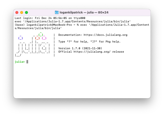 Julia 1.7 REPL after install
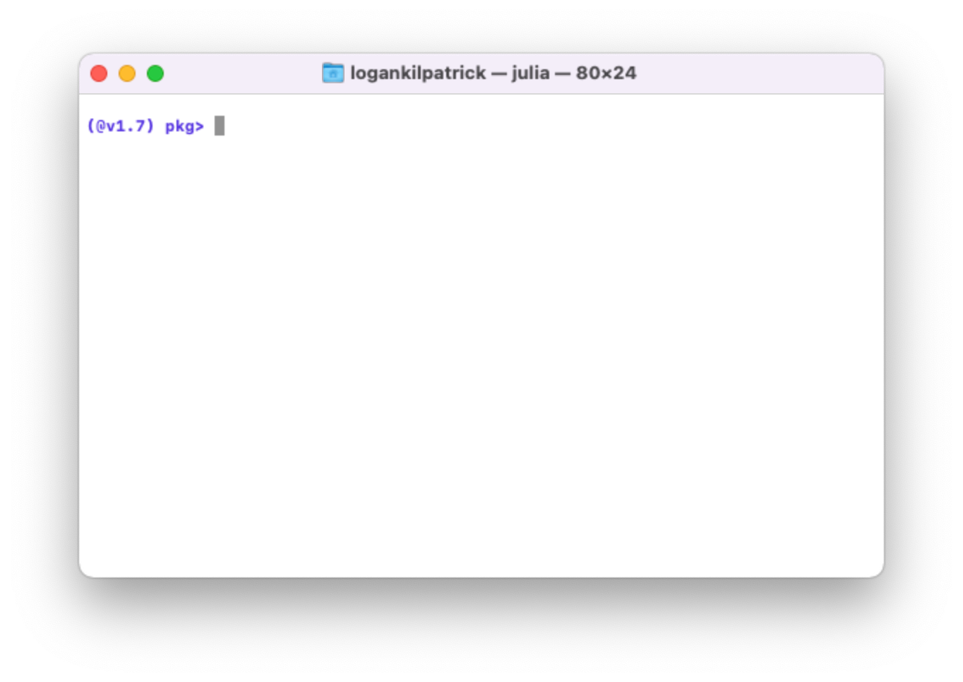 Pkg mode in the Julia REPL
Now that we are in the package manager, there are a few things we commonly want to do:
Pkg mode in the Julia REPL
Now that we are in the package manager, there are a few things we commonly want to do:
 If you recall, we removed the Flux package, and of course, I forgot this so I went to use it and load it in by typing